Johannes Schult

Scroll down for nice plots! Watch the video here!

This is a summary of the YouTube statistics of videos by the Vlogbrothers – Hank and John Green. The raw data were kindly provided by kitchensink108.tumblr.com. I focus on two dependent variables:

• Who made it? Hank-only, John-only, or both?
• The second variable of interest is the Date. In other words: When was the video put online?

The data set already contains a few interesting variables:

• The view count (Views)
• The number of Likes
• The number of Dislikes
• The number of Comments

The three latter numbers co-vary (all rank correlations > .7) with the total number of views, so looking at them all separately would be repetitive and boring. So instead I will look at:

• The view count – most of the time I’ll plot the natural logarithm of the view count because of a few outliers (more on those later)
• The Likes per View ratio (overall appreciation)
• The Likes per Dislike ratio (unambiguous appreciation)
• The Comments per View ratio along with the overall number of comments
• The length of the videos is not that interesting because most clock in just under 4 minutes. (NB: Longer videos were not included in the original data set.) There is just not enough variation. So I’ll just have one quick plot at the end.

Speaking of plots, most of the analysis will be graphical. This is pretty much a census, so there’s no need for statistical testing. Also, it’s all quite exploratory.

Here we go: Who tends to have more Views?

Here is the median view count for each brother: Hank: 256k, John: 286k, both: 347k. This means that 50% of Hank’s videos have more than 256k views, and the other half of his videos have less than 256k views. So John’s videos tend to get more views, but still less than reunion videos. You can also look at the means (M) and standard deviations (SD) – but there are some influential outliers that impede the interpretation of the numbers (Hank: M = 378k (SD = 537k); John: M =467k (SD = 1112k); both: M =367k (SD = 183k)).

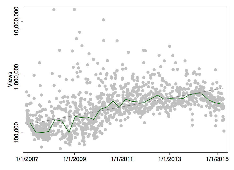
This plot shows the view count changes across time. The solid line is a median band. It indicates how many views a video needs at a given point in time to have less views than half of the other videos.

Each gray point represents one particular Vlogbrothers video. When I add the linear trend (actually, it’s a log-linear trend), it becomes clear that newer videos tend to get more views:

And this is the same plot with some additional Nerdfighter-related dates:

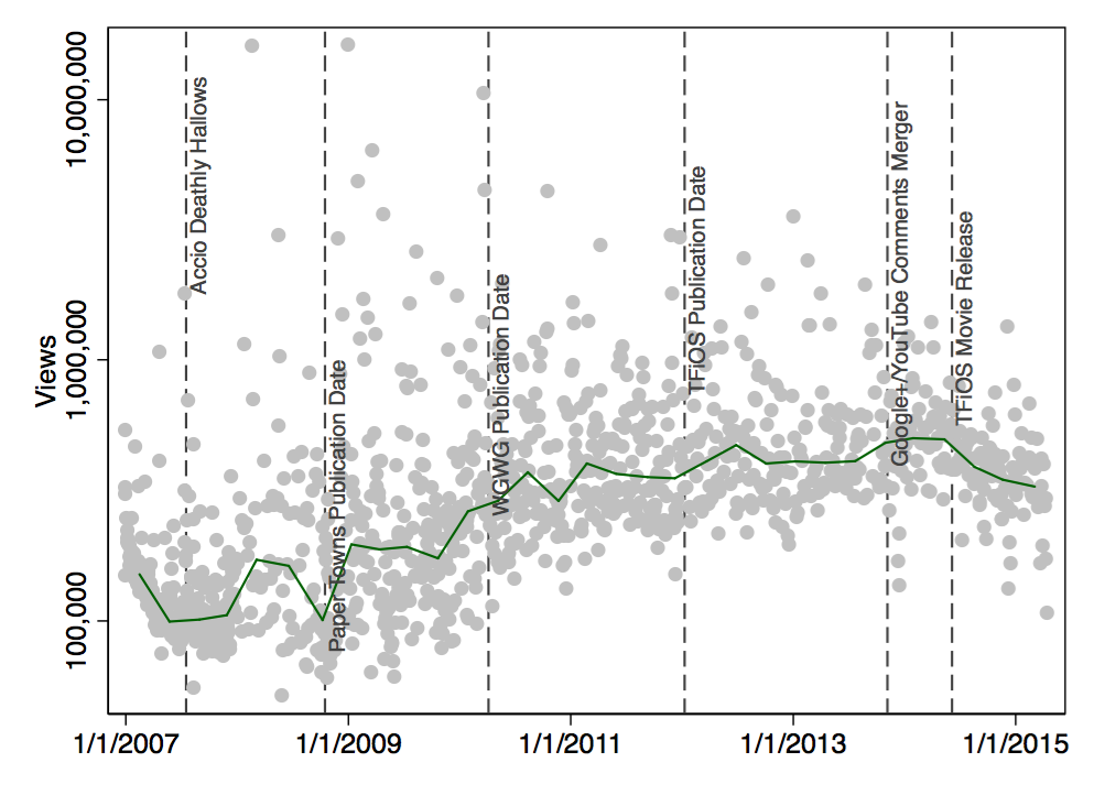
Did the movie version of The Fault in Our Stars lead to fewer views? I don’t think so – this is mostly speculation, anyway. There could be many reasons why Nerdfighters might be watching fewer videos (CrashCourse, SciShow, Tumblr, jobs, kids). Personally, I think that the more recent videos just haven’t accumulated as many views from new nerdfighters who go through old videos (and from random strangers).

Here is another version of this plot, this time with separate lines for John and Hank:

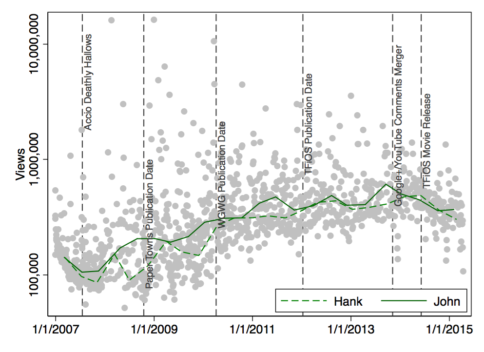
My interpretation would be that the view counts of Hank and John didn’t really develop differently.

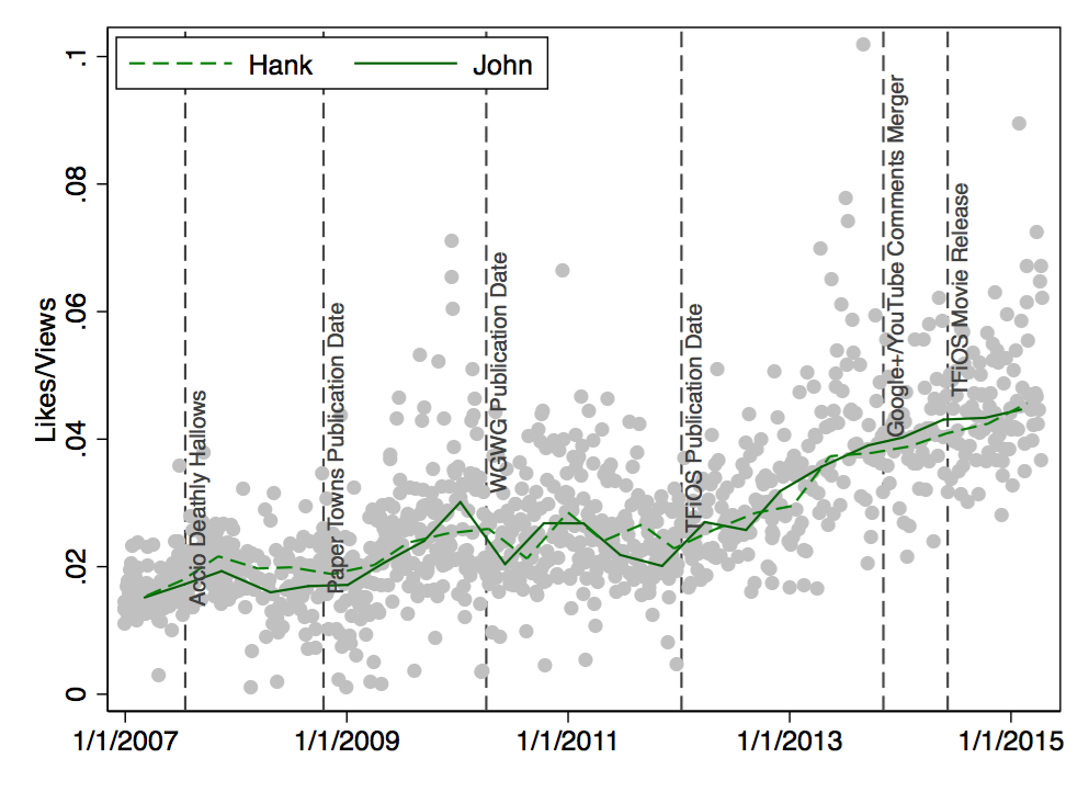
So far, so good. Now what about actual appreciation? When I look at the median values for Likes per View, Hank’s videos are liked by 2.3% of viewers. John’s videos are liked by 2.2% of viewers. Reunion videos are liked by 3.3%; Nerdfighters seem to like reunion videos!

Here’s the longitudinal perspective – again no clear differences between Hank’s videos and John’s videos:

Being liked is one thing. But how about the Likes per Dislike ratio? Here are the median values: Hank’s videos tend to get 78 Likes per Dislike. John’s videos tend to get 126 Likes for each Dislike. And reunion videos trumps them both with a median of 177 Likes per Dislike. Here’s the longitudinal perspective:

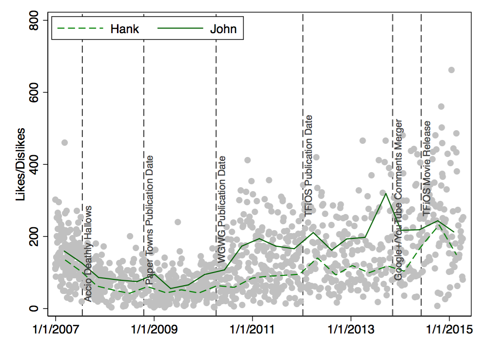
There were even more Likes than Dislikes during the past few years. This development occurred especially for John’s videos.

Enough with the appreciation – how about Comments? An eternal source of love, hate, fun, and chaos they are. The overall tendency (i.e., median) is that 0.5%-0.6% of viewers write a comment. Let’s look at the longitudinal perspective of Comments/Views:

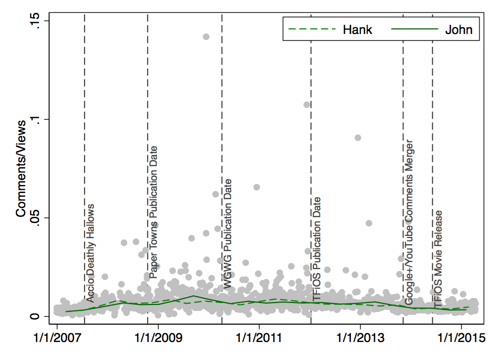
The number of Comments per View has declined over the past two years; possibly due to the integration of Google+ and YouTube or the new sorting algortihm for comments.

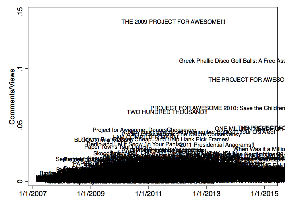
Finally, here’s a quick overview of specific types of outliers. Videos that elicit a lot of comments are mostly about the Project for Awesome:

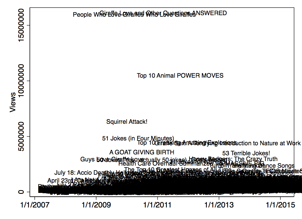
The videos with the highest view count all deal with animals:

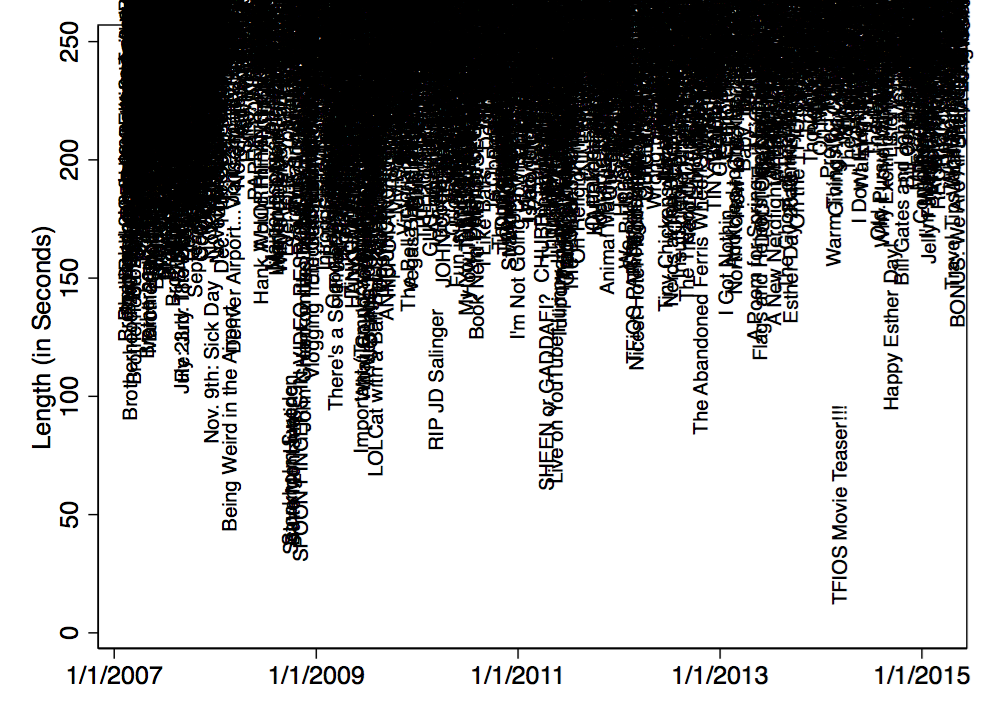
The last couple of plots brings us back to the length of the videos. Here are the titles of the shorter videos.

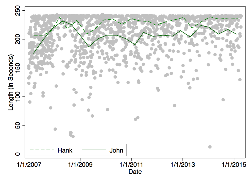
Not much to say here. And it seems as if Hank keeps making slightly longer videos than John:

That’s all. DFTBA!

PS a day later: I turned this post into a video. The initial text along with the analysis commands are listed in this Stata do-file.

fishingboatproceeds

[…] The same is true on amazon, where the book’s average rating has actually gone up a bit in the past six months (although not in a statistically significant way). […]

Actually, the ratings have decreased in a statistically significant way (alpha < .05). I used the two most recently archived pages from archive.org, which do not cover exactly 6 months. Still, ratings before 2013-02-03 were higher than those after that date.

• Before (2110 ratings): mean = 4.76 (SD = 0.014)
• After (1232 ratings): mean = 4.67 (SD = 0.021)

A t-test (two-sided, unequal variances) yields p = 0.0009 (d = -0.12); and for the non-parametric fans, the Wilcoxon rank-sum (Mann-Whitney) test yields p = 0.0001.

Using 2012-10-19 as dividing date, yields similar results:

• Before (1051 ratings): mean = 4.77 (SD = 0.020)
• After (2291 ratings): mean = 4.71 (SD = 0.015)

A t-test (two-sided, unequal variances) yields p = 0.0188 (d = -0.09); the Wilcoxon rank-sum test yields p = 0.0008. Of course, significance testing might be a questionable procedure in this case – and also in general.

This is actually a census of all Amazon ratings, so there’s no need to test whether ratings differ. The sample is the population. However, the written reviews could be regarded as a subsample of the ratings of all readers.

Is it a random sample? I don’t think so. So can we draw proper conclusions from the significance test results? Nah. I won’t provide a comprehensive discussion of the benefits and problems associated with the null hypothesis significance testing (NHST). I’ll just name one of my favourite objections, which Cohen (1990, p. 1308) phrased nicely: “The null hypothesis, taken literally (and that’s the only way you can take it in formal hypothesis testing), is always false in the real world.” In the present, the null hypothesis would mean, that average rating of newer readers is exactly the same as the average rating of those who pre-ordered the book etc.

Anyway, the effect size suggests that the drop in ratings is very small, so it should be safe to argue that the book keeps appealing to new readers.

PS: Sorry for nitpicking; this should in no way diminish the article, which I think is highly insightful.

PPS: I spend a good 15 minutes in R trying to beat the data into shape, but I feel much more comfortable in Stata, so I switched and had the analysis in a few minutes. Here’s the do-file in case anyone in curious. (Haha, as if!)

Continue reading ‘Null Hypothesis Significance Testing: The Fault in Our Stars’ »

The first round of the SpinTunes #3 song writing competition is over. Lo and behold, I made it to the next round! So needless to say I’m happy with the results. But equally important, the reviewers provided a lot of feedback. One is often inclined to retort when faced with criticism. Musicians even tend to reject praise if they feel misunderstood. I’m no exception. But this time around I actually agree with everything the judges wrote about my entry. (I Love the Dead – remember?) There wasn’t even the initial urge to provide my point of view, shed light on my original intentions. I will now go into the details, before I turn to a quick statistical analysis of the ratings in the last section of this post.

The incubation period for this song was rather long. At first, I was considering writing about the death metal band Death. It would have meant stretching the challenge and alienating anyone unfamiliar with the history of death metal (read: pretty much everyone). The only reminiscence of heavy metal in my actual entry is the adaptation of Megadeth’s “Killing Is My Business and Business Is Good”. I toyed with the idea of celebrating the death of a person who has lived fully and left nothing but happy marks on the lives others. Translating this idea into an actual song was a complete failure, though. I also considered writing about mortality statistics. There’s people who estimate the space needed for future graveyards and health insurances and so on. I’m somewhat familiar with the statistics behind that. But it would have taken weeks to turn this into a cohesive songs. So I returned to the notion of the happy grave digger. (Yes, Grave Digger is the name of a German metal band.) The working title was “Grave Digger’s Delight”. The music started with the chorus while I was playing an older idea I hadn’t used so far. Basically, I threw away the old idea except for the initial G-chord and the final change to D. I did add the intro melody, more on that soon. The verses are the good, old vi-IV-I-V, but with a ii thrown in for good measure. That’s not too original, but I was already running out of time. The lyrics started out with a word cloud of related terms. Plots With a View was a big inspiration when it came to the sincerity behind the mortician’s word. Here’s a person who’s dedicated to his job! I had wanted to include a couple of fancy funeral descriptions. But the music called for more concise lyrics. All that’s left from that idea is the line “I can give you silence – I can give you thunder”, which I kept to rhyme with “six feet under”. That one is indeed very plain, but I felt that the huge number of competitors called for a straight song that brings its message across during the first listen, preferably during the first 20 seconds. I think I succeeded in this respect. (This also a major reason why I changed the title to “I Love the Dead” – keeping it straight and plain.) The 2 minute minimum length gave me headaches. This made me keep, even repeat, the intro melody. I was tempted to use a fade out. But I always see this as a lack of ideas. So I used the working title for the ending. Given a few more days I might have come up with a more adequate closure. Even as I was filming the video, I felt the need to shorten the ending. I tried to spice up the arrangement with a bridge (post-chorus?) of varying length. I wasn’t completely sure about it during the recording process, but now I’m glad that the deadline forced me to keep it as it is. At one point I had a (programmed) drum track and some piano throughout the songs. To me it sounded as if they were littering the song rather than filling in lower frequencies. So I dropped them and just used a couple of nylon-stringed guitars (one hard right, one hard left), a steel-stringed guitar (center), a couple of shakers, lead vocals plus double-tracked vocals and harmony vocals in the chorus (slightly panned) and, of course, the last tambourine.

TL;DR – I appreciate the feedback and I resolve to start working on my next entry sooner.

Russ requests statistics. I happily obliged and performed a quick factor analysis using the ratings. What this method basically does is to create a multi-dimensional space in which the ratings are represented. There is one dimension for each judge, yielding a 9-dimensional space in the present case. If everybody judged the songs in a similar way, you would expect “good” songs to have rather high ratings on all dimensions the “bad” songs to receive low ratings. A line is fitted into this space to model this relationship. If all data point (i.e., songs) are close to that line in that space, the ratings are supposed to be uni-dimensionally.  In other words, there appears to be one underlying scale of song quality that is reflected in the ratings. This would be at odds with the common assertion that judgments are purely subjective and differ from rater to rater. (It would also suggest that computing the sum score is somewhat justified and not just creating numeric artifacts void of meaning.)

Using Stata 10 to perform a factor analysis with a principal-component solution, I get the following factors:

. factor blue-popvote, pcf
(obs=37)

Factor analysis/correlation                    Number of obs    =       37
Method: principal-component factors            Retained factors =        2
Rotation: (unrotated)                          Number of params =       17

--------------------------------------------------------------------------
Factor   |   Eigenvalue   Difference        Proportion   Cumulative
---------+----------------------------------------------------------------
Factor1  |      4.44494      3.29466            0.4939       0.4939
Factor2  |      1.15028      0.33597            0.1278       0.6217
Factor3  |      0.81431      0.08112            0.0905       0.7122
Factor4  |      0.73319      0.19850            0.0815       0.7936
Factor5  |      0.53468      0.05959            0.0594       0.8530
Factor6  |      0.47510      0.11760            0.0528       0.9058
Factor7  |      0.35750      0.05932            0.0397       0.9456
Factor8  |      0.29818      0.10635            0.0331       0.9787
Factor9  |      0.19183            .            0.0213       1.0000
--------------------------------------------------------------------------
LR test: independent vs. saturated:  chi2(36) =  137.45 Prob>chi2 = 0.0000

Wait, what? Let’s just focus on one criteria for exploring the factor solution: Eigenvalues larger than 1. Here are two such factors, which suggests that the rating data represents two (independent) dimensions. (For those familiar with the method: I tried a few rotated solutions, but they yield similar results.) Now the first factor explains almost half of the variance at hand whereas the second factor has a much smaller Eigenvalue and subsequently explains only 1/8 of the variance in the data.

Let’s take a look at the so called factor loading to see how the two factor relate to the raters. Stata says:

Factor loadings (pattern matrix) and unique variances

---------------------------------------------
Variable |  Factor1   Factor2 |   Uniqueness
---------+--------------------+--------------
blue     |   0.6128   -0.0039 |      0.6244
mike     |   0.7690   -0.1880 |      0.3733
mitchell |   0.7188    0.1032 |      0.4727
glenn    |   0.7428   -0.0309 |      0.4474
randy    |   0.8830    0.0089 |      0.2202
kevin    |   0.7768    0.1219 |      0.3817
david    |   0.6764    0.3650 |      0.4092
ben      |  -0.0672    0.9439 |      0.1045
popvote  |   0.7512   -0.2534 |      0.3714
---------------------------------------------

Without going into statistical details, let’s say that the loading indicate who strongly each rater is related with each factor. For example, Blue’s ratings have less to do with the overall factor than Mike’s ratings. Both rater’s show rather high loadings, though. Given the high loading of all raters (except one) indicate a high level of general agreement. The only exception is Ben, whose ratings have little to do with the first factor. (You could argue that he even gave reverse ratings, but the loading is quite small.) Instead, his ratings play a big role in the second factor (which is by definition statistically independent from the first one). There is some agreement with the remaining variance of David’s ratings and a negative relationship with the popular vote (if you use the somewhat common notion to interpret loadings that are larger than 0.2). So there appears to be some dissent regarding the ranking. But on the other hand, the “dominant” first factor suggests that the ratings reflect the same construct to a large degree. Whether that’s song writing skills, mastering of the challenge, or simply sympathy, is different question.

PS: I must admit that I haven’t listened to all entries, yet. It’s a lot of music and I’m struggling with a few technical connection glitches. Anyway, I liked what Jason Morris and Alex Carpenter did, although their music wasn’t that happy. Another entry that necessarily caught my attention was Wake at the Sunnyside by the one and only Gödz Pöödlz. Not only did they choose the same topic I used, they also came up with a beautiful pop song and plenty of original lyrical ideas. Good work!

My current research requires meta-analytic procedures where variables that contain another variable’s mean come in very handy. Centering Variables is also something very reasonable to do when analysing regressions with an interaction term between a continuous variable and a dummy variable.

Centering variables sounds like an easy task. It is if you use Stata but I found it surprisingly difficult in SPSS (unless you enter the means by hand, which is error-prone and impractible for repeated analyses). Here’s how you can calculated a variable which contains the mean of another variable (which can then easily be centered or used in whatever way one wants to).

Let dres be the variable of interest. The new variable containing the mean of dres (for all obversations) will be named dresavg. I also show how to create a variable containing the number of observations (ntotal). cdres will be the centered variable.

Stata 10

Use

. egen dresavg = mean(dres)

and you’re done! You could also use summarize and generate commands:

. sum dres
. gen dresavg = r(mean)

If you want a variable that contains the total number of observations you can use

. gen ntotal = _N

or with the more flexible egen command (e.g., handy when dres has missings)

. egen ntotal = count(dres)

There are plenty ways to generate various variables containing sample statistics. As for the centered variable, use

. gen cdres = dres - dresavg

or without even generating the variable containing the mean:

. sum dres
. gen cdres = dres - r(mean)

PASW 18 (SPSS, you know)

Beware, long syntax ahead. Before you despair, there’s a simpler (but less flexible) solution below. The complicated approach starts with exporting the variable mean into a new data set. This data set is then merged with the master data set; a variable containing the mean for every observation will be attached. Continue reading ‘Practical tips for statisticians (part 8): centering variables using Stata and SPSS’ »

A couple of days ago I got hold of the book The Workflow of Data Analysis Using Stata by J. Scott Long. I haven’t yet delved into it. But I’m already loving and condemning it. Loving it, because it covers an integral part of scientific data analysis, filling a void that left by both the literature and the courses taught at university. Condemning it, because I had wanted to write a book on the same topic (how to ensure your data analysis is documented well, i.e., replicable) during the next years. It wouldn’t have been the same book; in fact, it would have been vastly different, possibly much worse.

It’s too early for me to review the book in a conclusive manner. Still, the content looks very promising and I think it’s telling that Long focuses on Stata as the software of choice. This is going to be fun!